Semi-Supervised Learning Using Gaussian Fields and Harmonic Functions
This is the very first blog I have written in 2023. This collection of blogs are all about famous literature (classics) in graph learning, causal inference, and data science. By writing these blogs, my aim is to learn and collect insights that are often overlooked in our study of “neural nets-based ML” and to rethink the potential of traditional statistical models and methods.
Keywords: Gaussian Fields, Harmonic Functions, Semi-Supervised Learning, Graph Smoothing.
Summary
This paper is about the task to perform semi-supervised learning on graphs. In specific, labelled and unlabelled data are represented as nodes in a weighted graph, with edges weights encoding the similarity between nodes.
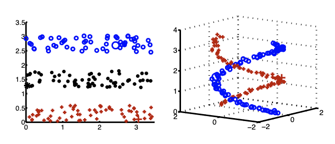
This paper illustrates the fundamental motivation for using a graph representation: smoothness. In reality, we always face the curse of dimensionality–the phenomenon that high-dimensional data is unavoidably sparse. Graph smoothing is an important way to tackle this issue. Intuitively, smoothing allows the model to infer an unseen data point by relating it to the seen ones. The idea that nodes with connections share similarity is sometimes also referred to as homophily, and is the key assumption in most current research on Graph Neural Networks.
Problem Formulation
We suppose there are $l$ labeled points $\left(x_1, y_1\right), \ldots,\left(x_l, y_l\right)$, and $u$ unlabeled points $x_{l+1}, \ldots, x_{l+u}$; typically $l \ll u$. Let $n=l+u$ be the total number of data points. To begin, we assume the labels are binary: $y \in\{0,1\}$. Consider a connected graph $G=(V, E)$ with nodes $V$ corresponding to the $n$ data points, with nodes $L=\{1, \ldots, l\}$ corresponding to the labeled points with labels $y_1, \ldots, y_l$, and nodes $U=\{l+1, \ldots, l+u\}$ corresponding to the unlabeled points. Our task is to assign labels to nodes $U$. We assume an $n \times n$ symmetric weight matrix $W$ on the edges of the graph is given. For example, when $x \in \mathbb{R}^m$, the weight matrix can be [ w_{i j}=\exp \left(-\sum_{d=1}^m \frac{\left(x_{i d}-x_{j d}\right)^2}{\sigma_d^2}\right) ] where $x_{i d}$ is the $d$-th component of instance $x_i$ represented as a vector $x_i \in \mathbb{R}^m$, and $\sigma_1, \ldots, \sigma_m$ are length scale hyperparameters for each dimension. Thus, nearby points in Euclidean space are assigned large edge weight.
Our strategy is to first compute a real-valued function $f: V \longrightarrow \mathbb{R}$ on $G$ with certain nice properties, and to then assign labels based on $f$. We constrain $f$ to take values $f(i)=f_l(i) \equiv y_i$ on the labeled data $i=1, \ldots, l$. Intuitively, we want unlabeled points that are nearby in the graph to have similar labels. This motivates the choice of the quadratic energy function [ E(f)=\frac{1}{2} \sum_{i, j} w_{i j}(f(i)-f(j))^2 ]
Harmonic Property
As the author points out, it is “not difficult” to show that the minimum energy function (constrained on labelled nodes) is harmonic (The value of $f$ at each unlabelled data point is the average of $f$ at neighboring nodes.). The following are the equivalent definitions of harmonic property:
- $\Delta f = (D-W)f=0$, where $\Delta$ is the combinatorial Laplacian.
- $f(j)=\frac{1}{d_j} \sum_{i \sim j} w_{i j} f(i)$, for $j=l+1, \ldots, l+u$
- $f=Pf=(D^{-1}W)f$.
Letting $f=\left[\begin{array}{c}f_l \\ f_u\end{array}\right]$ where $f_u$ denotes the values on the unlabeled data points, the harmonic solution $\Delta f=0$ subject to $f\mid_L=f_l$ is given by [ f_u=\left(D_{u u}-W_{u u}\right)^{-1} W_{u l} f_l=\left(I-P_{u u}\right)^{-1} P_{u l} f_l ]
Interpretation and Connections
- Electric networks: Imagine the edges of $G$ to be resistors with conductance $W$. The nodes labelled to corresponding voltage sources ($1V$ or ground). The $f_u$ is just the resulting voltage at the unlabelled nodes.
- Graph kernel
- Spectral Clustering and Graph Mincuts
Incorporating Prior Knowledge
The problem stems from the fact that $W$, which specifies the data manifold, is often poorly estimated in practice and does not reflect the classification goal. In other words, we should not “fully trust” the graph structure. Therefore, we can adjust the harmonic threshold according to some prior knowledge about the desirable class proportions. This method extends naturally to the general multiclass case.
Incorporating External Classifiers
Often we have an external classifier at hand, which is constructed on labeled data alone. In this section we suggest how this can be combined with harmonic energy minimization. Assume the external classifier produces labels $h_u$ on the unlabeled data; $h_u$ can be $0 / 1$ or soft labels in $[0,1]$. We combine $h_u$ with harmonic energy minimization by a simple modification of the graph. For each unlabeled node $i$ in the original graph, we attach a “dongle” node which is a labeled node with value $h_i$, let the transition probability from $i$ to its dongle be $\eta$, and discount all other transitions from $i$ by $1-\eta$. We then perform harmonic energy minimization on this augmented graph. Thus, the external classifier introduces “assignment costs” to the energy function, which play the role of vertex potentials in the random field. It is not difficult to show that the harmonic solution on the augmented graph is, in the random walk view, [ f_u=\left(I-(1-\eta) P_{u u}\right)^{-1}\left((1-\eta) P_{u l} f_l+\eta h_u\right) ]
Reference
Xiaojin Zhu, Zoubin Ghahramani, and John Lafferty. 2003. Semi-supervised learning using Gaussian fields and harmonic functions. In Proceedings of the Twentieth International Conference on International Conference on Machine Learning (ICML’03). AAAI Press, 912–919.